AP Statistics : Properties of Single Sample Distributions
Study concepts, example questions & explanations for AP Statistics


All AP Statistics Resources
Example Questions
Example Question #111 : Statistical Patterns And Random Phenomena
Suppose that the mean height of college students is 70 inches with a standard deviation of 5 inches. If a random sample of 60 college students is taken, what is the probability that the sample average height for this sample will be more than 71 inches?


First check to see if the Central Limit Theorem applies. Since n > 30, it does. Next we need to calculate the standard error. To do that we divide the population standard deviation by the square-root of n, which gives us a standard error of 0.646. Next, we calculate a z-score using our z-score formula:
}{S.E.}")

Plugging in gives us:
}{0.646} = 1.548")
Finally, we look up our z-score in our z-score table to get a p-value.
The table gives us a p-value of,
=1-P(z<1.58) \\P(z>1.58)=1-0.9394 \\P(z>1.58)=0.0606")
Example Question #11 : Properties Of Single Sample Distributions
A random variable has an average of 


There are two keys here. One, we have a large sample size since 
Our 
}{\sqrt{n} \cdot \sigma}")
where 


and 
}{\sqrt{80} \cdot 5}=0.8944")
 = 0.8133")
Example Question #11 : Properties Of Single Sample Distributions
Let us suppose we have population data where the data are distributed Poisson
(see the figure for an example of a Poisson random variable). 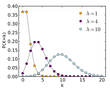
Which distribution increasingly approximates the sample mean as the sample size increases to infinity?
Gamma
Poisson
Normal
Exponential
Normal
The Central Limit Theorem holds that for any distribution with finite mean and variance the sample mean will converge in distribution to the normal as sample size 

Example Question #2 : How To Use The Central Limit Theorem
Cat owners spend an average of $40 per month on their pets, with a standard deviation of $5.
What is the probability that a randomly selected pet owner spends less than 


First, draw the distribution and the area you are interested in.
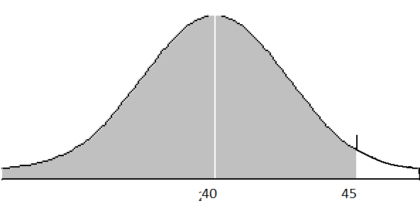
Next, calculate the z-score for the person of interest. Because the population standard deviation is known, we will use the formula for z-score and not t-score.
We will find the z-score for the person of interest, and then calculate the area under the curve that falls below, or to the left of that z-score.

Now we will find the value for each variable given in the problem:


Third, solve for z using the information in the problem.


Now we must determine the area under the curve to the left of a z-score of 1.0. We will consult a z-table.
Look up 1.0 in the row and 0.00 in the column.
If your z-table gives shaded area to the left, you will get
=0.8413")
We are interested in area to the left, which is what we found, so this is our answer.
If your z-table gives shaded area to the right, you will get
=0.1587")
Because we want the area to the left of z=1.0, we will subtract that area from 1:

Example Question #2 : How To Use The Central Limit Theorem
It is known that cat owners spend an average of 

What is the probability that a randomly selected cat owner spends between 


First, draw the distribution and the area you are interested in.
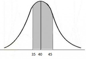
Next, we will need to calculate z-scores for both values we are interested in, and find the area under the curve that falls between these two values.
Because the population standard deviation is known, we will use the formula for z-score and not t-score.

We will find the z-score for the lower bound and find the z-score for the upper bound.
For the lower bound:


Now we will do the same for the upper bound:


Now we must determine the area under the curve which falls between z-scores of -1.0 and 1.0. To do this we will look up both z-scores and then subtract their areas (subtract the smaller area from the bigger area, so that you don't get a negative value).
For the lower bound, look up 1.0 in the row and 0.00 in the column. Then, for the upper bound, look up -1.0 in the row and 0.00 in the column.
The area to the left of 1.0 is 0.8413.
The area to the left of -1.0 is 0.1587.
To find the area between the two z-scores just subtract:

The central limit theorem states that the area under the curve + or - 1 standard deviation from the mean is 68.3%, which we have confirmed.
Example Question #112 : Statistical Patterns And Random Phenomena
Cat owners spend an average of 

What is the probability that a randomly chosen cat owner spends more than 


First, draw the appropriate curve to represent the problem: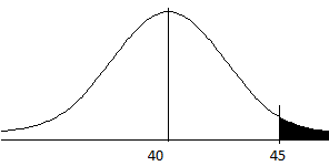
Because we want greater than 45, shade the right hand portion of the graph.
We will be using the z-distribution and not the t-distribution because we know the population standard deviation.
We will find the z-score for this cat owner, and then find the area to the right of that z-score to find the probability of spending more than $45.
We begin with the z-score formula:

Now find each value from the information given:


Fill in the formula


Now look this z-score up in the z-table to find the area under the curve. Look up 1.0 in the row and 0.00 in the column.
If your z table gives area shaded to the left, you will find
= 0.8413")
You want the area to the right, so subtract the above from 1.

If your z table gives area shaded to the right, you will find
= 0.1587")
Because you want the area to the right of z=1.0, this is your answer.
Example Question #113 : Statistical Patterns And Random Phenomena
If the Central Limit Theorem applies, we can infer that:
Every possible sample mean will be equal to the population mean.
The sample mean will be close to the population mean.
The standard deviation will be small.
The sampling distribution will be approximately normally distributed.
The sampling distribution will be approximately normally distributed.
The Central Limit Theorem tells us that when the theorem applies, the sampling distribution will be approximately normally distributed.
Example Question #12 : Properties Of Single Sample Distributions
A survey company samples 60 randomly selected college students to see if they own an American Express credit card. One percent of all college students own an American Express credit card. Does the Central Limit Theorem apply?
No.
Yes.
Not enough information is given.
No.
No. Whenever we get a "proportion" question we need to check whether 
\geq10")
In this problem, 
Therefore,

So the central limit theorem does not apply.
Example Question #4 : How To Use The Central Limit Theorem
In a particular library, there is a sign in the elevator that indicates a limit of 


If a random sample of 


None of the other answers


This question deals with the Central Limit Theorem, which states that a random sample taken from a large population where the sampling distribution of sample averages is approximately normal has a standard deviation equal to the standard deviation of the population divided by the square root of the sample size. The information given allows us to apply the Central Limit Theorem as it satisfies the necessary characteristics of the sampling distribution/size. The standard deviation of the population is 27lbs, and the sample size is 36; therefore, the standard deviation of the 36-person random sample is 


All AP Statistics Resources